How to Find the Min of a Array Using Merge Sort

Merge Sort Algorithm

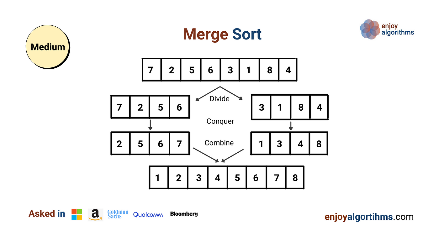
Difficulty

Medium

Asked In

Microsoft, Amazon, Goldman Sachs, Qualcomm, Bloomberg, Paytm

Why Merge Sort?

Merge sort is a popular sorting algorithm that uses a divide and conquer approach to sort an array (or list) of integers (or characters or strings). Here are some excellent reasons to learn this algorithm -

One of the efficient sorting algorithms that work in O(nlogn) time complexity in the worst case.
The best algorithm for sorting linked lists, i.e., can sort the linked list in O(nlogn) time complexity in the worst case.
An excellent algorithm to learn recursion and its analysis. We can use a similar recursive approach to solve other coding questions.
The merging algorithm used in the merge sort is a good idea to learn problem-solving using two-pointers. Here both the pointers are moving in the same direction to build the partial solution. We can use an approach to solve other coding questions.

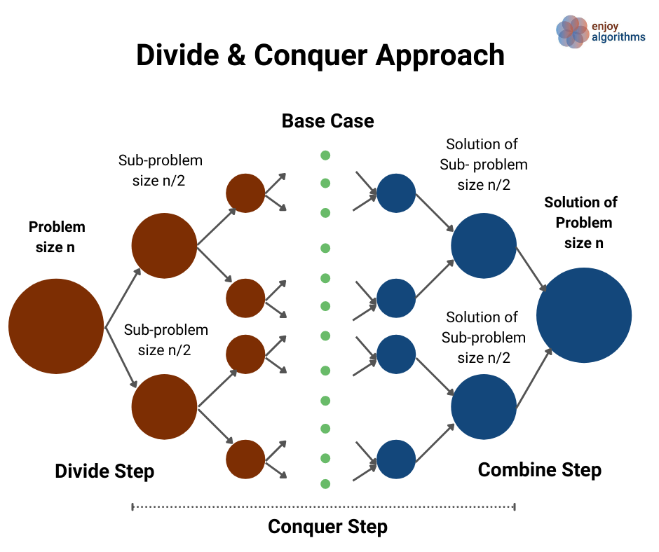
Merge Sort Idea

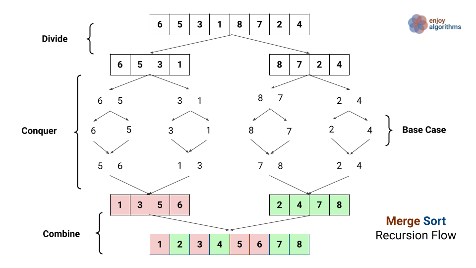
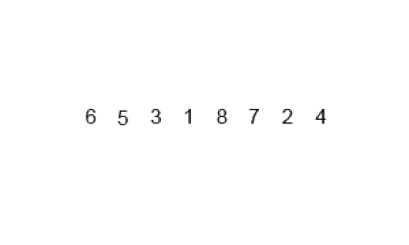
Suppose we need to sort an array A[l…r] of n integers starting from index l and ending at index r. Now a critical question would be — how do we solve the sorting problem using smaller sub-problems by applying the divide and conquer approach? Let's think!

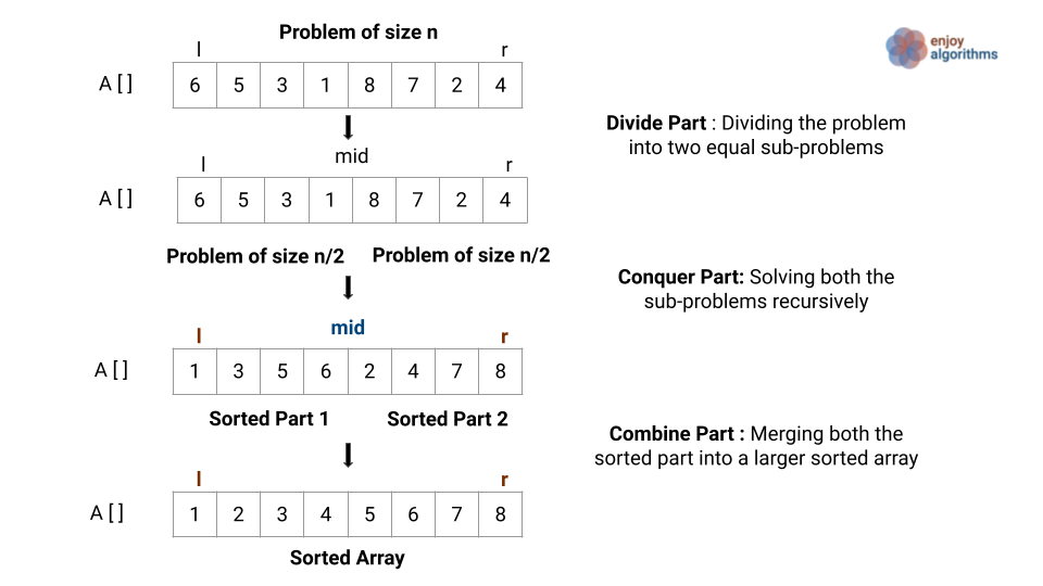
If we observe from the above diagram, the idea of merge sort will go like this:

Divide part — divide the sorting problem of size n into two different and equal sub-problems of size n/2. We can easily divide the problem by calculating the mid-value.

Left Subproblem — sorting array A[] from l to mid
Right Subproblem — sorting array A[] from mid+1 to r

Conquer Part — Now, solve both the sub-problems recursively. We need not worry about the solutions to the sub-problems because recursion will do this work.

Combine Part — We combine solutions of both the sub-problems of size n/2 to solve the sorting problems of size n. In simple words, we merge both sorted halves to generate the final sorted array. How? Think!

Merge Sort Steps

Suppose the function mergeSort(int A[], int l, int r) sort the entire array A[] where we are passing the left index l and right index r as an input parameter.

Divide Part : Calculating the mid-value, mid = l + (r — l)/2
Conquer Part 1: Recursively calling the same function to sort the left half of input size n/2, i.e., mergeSort(A, l, mid). We are passing mid as the right index.
Conquer Part 2: Recursively calling the same function to sort the right half of input size n/2, i.e., mergeSort(A, mid+1, r). We are passing mid +1 as the left index.
Combine Part: Inside the function mergeSort(), we use the function merge(A, l, mid, r) to merge both the sorted halves into a single sorted array.
Base Case: If we find l==r during the recursive calls, then the sub-array has at most one element left, which is already sorted. Our recursion will not go further and return from here. In other words, The sub-array of size one is the smallest version of the sorting problem for which recursion directly returns the solution.

Merge Sort pseudo code

          void mergeSort(int A[], int l, int r)
{
            if(l >= r)
            return
            int mid = l + (r - l)/2
            mergeSort(A, l, mid)
            mergeSort(A, mid + 1, r)
            merge(A, l, mid, r)
}

Merge Sort Visualisation

Combine Part — The merging algorithm

Merging algorithm idea: Two Pointers

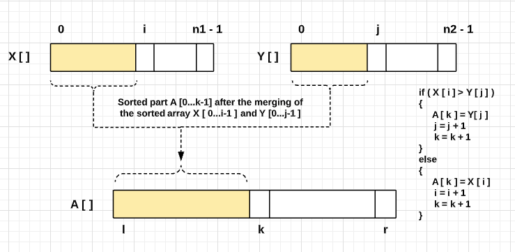
After the conquer step, both left part A[l…mid] and right part A[mid+1…r] will be sorted. Now we need to combine the solution of the two smaller sub-problems to build the solution of the larger problem, i.e., merge two sorted halves to create a larger sorted array. How can we do it? Let's think. But one thing is sure — we cannot merge these two sorted parts in place! (Think!)

If we store the values of both sorted halves of A[] into two extra arrays of size n/2 (X[] and Y[]), then we can transform the problem into — merging sorted arrays X[] and Y[] to the larger sorted array A[]. Now using the sorted order property and comparing the values one by one in both the arrays, we can build the larger array sorted A[]. How we implement it? Let's think!

We can use two separate pointers i and j, to traverse the array X[] and Y[] from the start. We compare elements in both the arrays during the traversal and place a smaller value on the larger array A[]. Another way of thinking would be — after each comparison, we add one input to the output and build the partially sorted array A[]. (Think!)

Merging algorithm steps

Step 1: Memory allocation and data copy process

We first calculate the size of left and right-sorted parts, including value at mid-index to the left part. Size of left part (n1) = mid — l +1, Size of right part (n2) = r — mid. Now we allocate the two extra arrays, X[] and Y[], of sizes n1 and n2 and copy the left and right sorted parts of A[] in both the arrays.

          int n1 = mid - l + 1
int n2 = r - mid
int X[n1], Y[n2]
for (int i = 0; i < n1; i = i + 1)
            X[i] = A[l + i]
for (int j = 0; j < n2; j = j + 1)
            Y[j] = A[mid + 1 + j]

Step 2: Merging algorithm loop

We initialises the loop pointers i, j, and k to traverse the array X[], Y[], and A[] i.e. i = 0, j = 0 and k = l. In other words, we start from the smallest element of both sorted arrays! Now we run a loop until any smaller arrays reach its end: while(i < n1 and j < n2). At the first step of the iteration, we compare X[0] and Y[0] and place the smallest value at A[0].

Before moving forward to the second iteration, we increment the pointer k in A[] and pointer in the array containing the smaller value(It may be i or j, which depends on the comparison.Think!). Similarly, we move forward in all three arrays using pointers i, j, and k. At each step, we compare X[i] & Y[j], place a smaller value to A[k], and increment the value of k by 1. Based on the comparison and position of the smaller value, we also increment the pointers i or j.

Note: This is a two-pointer approach of problem-solving where we build the partial solution by moving pointer i and j in the same direction.

          while (i < n1 && j < n2)            
{
            if (X[i] <= Y[j])            
            {
            A[k] = X[i]
            i = i + 1
            }
            else            
            {
            A[k] = Y[j]
            j = j + 1
            }
            k = k + 1
}

merge sort algorithm two pointer approach of the merging process

Step 3: Loop termination and boundary conditions

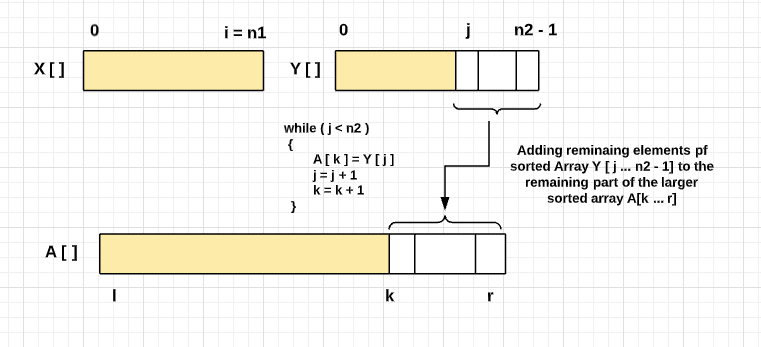
We exit the loop when any one of the two pointers reaches its end (either i = n1 or j = n2).

Boundary Condition 1 — If we exit the loop due to condition j = n2, then we reached the end of the sorted array Y[] and placed all the values of Y[] in A[]. But there may be some values remaining in X[] which still need to put in the larger sorted array. We copy all the remaining values of X[] in the larger array A[].Why? Think!

          while (i < n1)            
{
            A[k] = X[i]
            i = i + 1
            k = k + 1
}

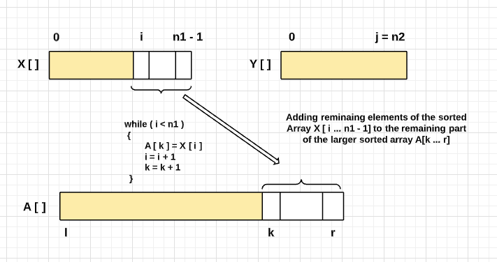
merge sort algorithm merging process termination 1

Boundary Condition 2 — If we exit the loop due to condition i = n1, then we reached the end of the sorted array X[] and placed all the values of X[] in A[]. But there may be some values remaining in Y[] which still need to put in the larger sorted array. We copy all the remaining values of Y[] in the larger array A[].

          while (j < n2)            
{
            A[k] = Y[j]
            j = j + 1
            k = k + 1
}

merge sort algorithm merging process termination 2

Merging algorithm Pseudocode

          void merge(int A[], int l, int mid, int r)
{
            int n1 = mid - l + 1
            int n2 = r - mid
            int X[n1], Y[n2]
            for (int i = 0; i < n1; i = i + 1)
            X[i] = A[l + i]
            for (int j = 0; j < n2; j = j + 1)
            Y[j] = A[mid + 1 + j]                      int i = 0, j = 0, k = l
            while (i < n1 && j < n2)            
            {
            if (X[i] <= Y[j])            
            {
            A[k] = X[i]
            i = i + 1
            }
            else            
            {
            A[k] = Y[j]
            j = j + 1
            }
            k = k + 1
            }                  while (i < n1)              
              {
              A[k] = X[i]
              i = i + 1
              k = k + 1
              }
              while (j < n2)              
              {
              A[k] = Y[j]
              j = j + 1
              k = k + 1
              }
}

Time and Space complexity of merging algorithm

This is an excellent code to understand the time complexity of the iterative algorithm. To understand this better, let's visualize the time complexity of each critical step and do the sum to calculate the overall time complexity.

Memory allocation = O(1)
Data copy process = O(n1) + O(n2) = O(n1 + n2) = O(n)
Inner while loop (In the worst case) = O(n1 + n2) = O(n)
Boundary condition 1 (In the worst case) = O(n1)
Boundary condition 2 (In the worst case) = O(n2)
Overall Time Complexity = O(1)+ O(n) + O(n) + O(n1) + O(n2) = O(n)

If we observe closely, then the merging algorithm time complexity depends on the inner while loop where comparison, assignment, and increment are the critical operations. There could be two different perspectives to understand this analysis:

Perspective 1: At each step of the while loop, we increment either pointer i or j. In all situations, we have to traverse both arrays until the end.
Perspective 2: At each step of the iteration, we place each element of the smaller sorted arrays to the larger array A[].

Space Complexity = extra space of size n/2 for storing the left part + extra space of size n/2 for storing the right part = O(n1) + O(n2) = O(n1 + n2) = O(n)

Time and Space complexity of the merge sort

Let's assume that T(n) is the worst-case time complexity of merge sort for n integers. When we have n>1 (merge sort on a single element takes constant time), then we can break down the time complexities as follows:

Divide Part: The time complexity of the divide part is O(1) because calculating the middle index takes constant time.
Conquer Part: We are recursively solving two sub-problems, each of size n/2. So the time complexity of each subproblem is T(n/2) and the overall time complexity of the conquer part is 2T(n/2).
Combine Part — As calculated above, the worst-case time complexity of the merging process is O(n).

For calculating the T(n), we need to add the time complexities of the divide, conquer, and combine part=> T(n) = O(1) + 2 T(n/2) + O(n) = 2 T(n/2) + O(n) = 2 T(n/2) + cn

T (n) = c, if n = 1
T(n) = 2 T(n/2) + cn, if n > 1

Note: Our merge sort function works correctly when the number of elements is not even. But to simplify the analysis, we assume that n is a power of 2 where the divide step creates the sub-problems of size exactly n/2. This assumption does not affect the order of growth of the analysis. (Think!)

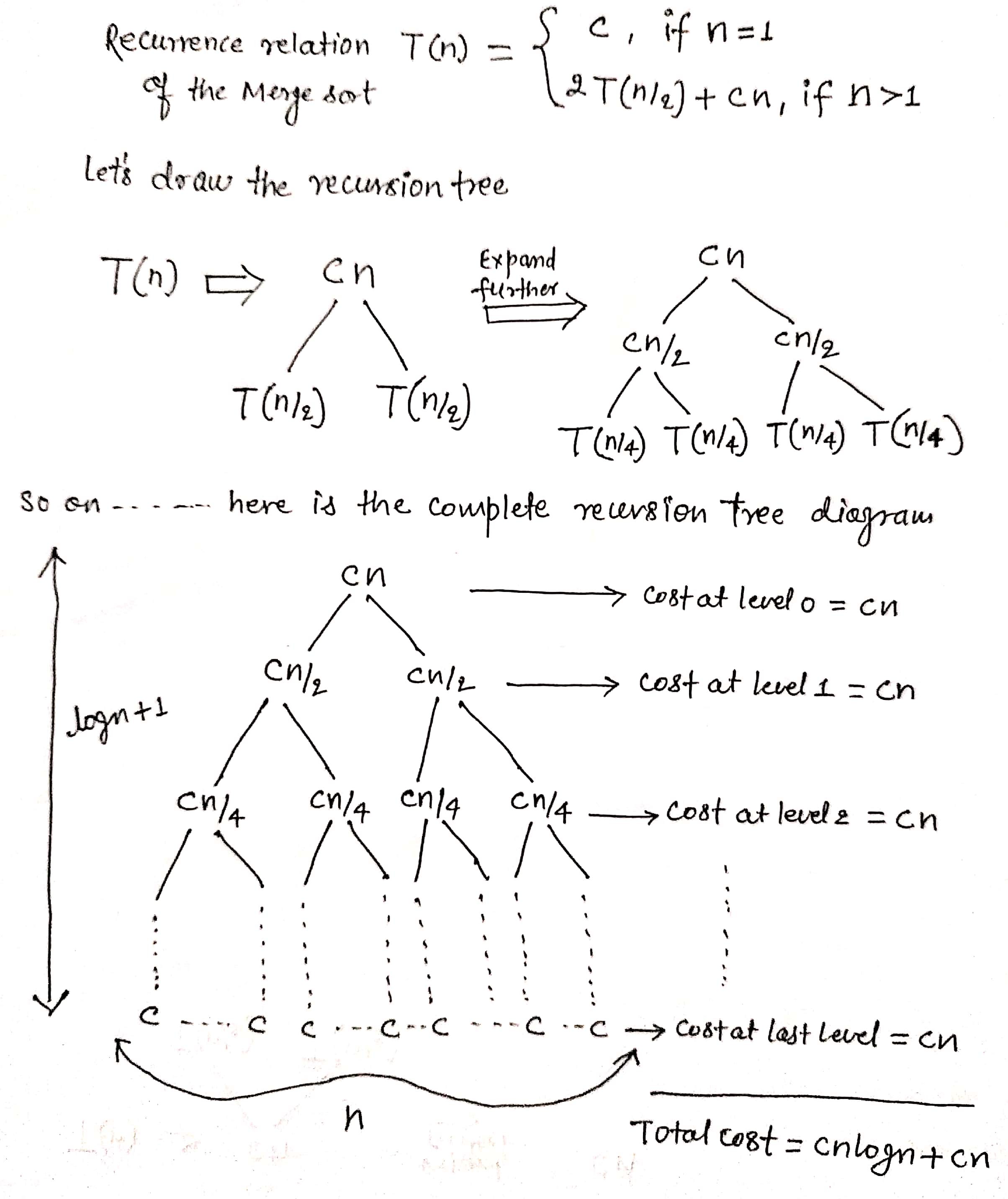
Analysis using the recursion tree method

In this method, we draw a recursion tree and count the total number of operations at every level. Finally, we find the overall time complexity by doing the sum of operations count at each level.

Analysis using the master theorem

Master method is a direct way to get the solution for the recurrences that can be transformed to the type T(n) = aT(n/b) + O(n^k), where a≥1 and b>1. There are the following three cases of the analysis using master theorem:

If f(n) = O(n^k) where k < logb(a) then T(n) = O(n^logb(a))
If f(n) = O(n^k) where k = logb(a) then T(n) = O(n^k * logn)
If f(n) = O(n^k) where k > logb(a) then T(n) = O(n^k)

          Let's compare with the merge sort recurrence
- T(n) = 2 T(n/2) + cn, if n > 1
- T(n) = aT(n/b) + O(n^k)          Here a = 2, b = 2 (a > 1 and b > 1)
=> O(n^k)= cn = O(n¹) => k = 1          Similarly, logb(a) = log 2(2) = 1
Hence => k = logb(a) = 1          It means, Merge sort recurrence satisfy            
the 2nd case of the master theorem.          Time complexity T(n)            
= O(n^k * logn)            
= O(n^1 * logn)            
= O(nlogn)

Space complexity of merge sort = space complexity of the merging process + size of recursion call stack = O(n) + O(logn) = O(n). Note: size of recursion call stack = height of the merge sort recursion tree = O(logn) (Think!)

Critical ideas to think in merge sort!

Merge sort is a stable sorting algorithm that means that identical elements are in the same order in the input and output.
For the smaller input, It is slower in comparison to other sorting algorithms. Even it goes through the complete process if the array is already or almost sorted.
Merge sort is the best choice for sorting a linked list. It is relatively easy to implement a merge sort in this situation to require only O(1) extra space. On the other hand, a linked list's slow random-access performance makes some other algorithms, such as quicksort, perform poorly and others like heap sort completely impossible.
We can parallelize the merge sort's implementation due to the divide-and-conquer method, where every smaller sub-problem is independent of each other.
The multiway merge sort algorithm is very scalable through its high parallelization capability, which allows many processors. This makes the algorithm a viable candidate for sorting large amounts of data, such as those processed in computer clusters. Also, since memory is usually not a limiting resource in such systems, the disadvantage of space complexity of merge sort is negligible.
We can implement merge sort iteratively without using an explicit auxiliary stack. On another side, recursive merge sort uses function call stack to store intermediate values of function parameters l and r and other information. The iterative merge sort works by considering window sizes in exponential oder, i.e., 1,2,4,8..2^n over the input array. For each window of any size k, all adjacent pairs of windows are merged into a temporary space, then put back into the array. Explore and Think! We will write a separate blog on this.

Mungomery Callibed